Paper-Review of “Graph Neural Controlled Differential Equations for Traffic Forecasting”

1. Introduction

Recent advances in data acquisition technology help collect a variety of spatio-temporal (ST) data in urban areas, such as urban traffic, air quality, and etc. Such data has complex spatial and temporal correlations, which can be depicted by spatio-temporal graphs(STG), as shown in Fig. 1. For example, spatio-temporal data describes various things and movements as $[x, y, h, t]$. Take the geodetic coordinate system (rectangular coordinate system) as an example to describe, that is $[longitude, latitude, altitude, time]$. This can describe almost all kinds of things. As small as the trajectory of a car, the process of building construction, and as large as the movement of plates, they can all be abstracted as $[x, y, h, t]$.

picfig3

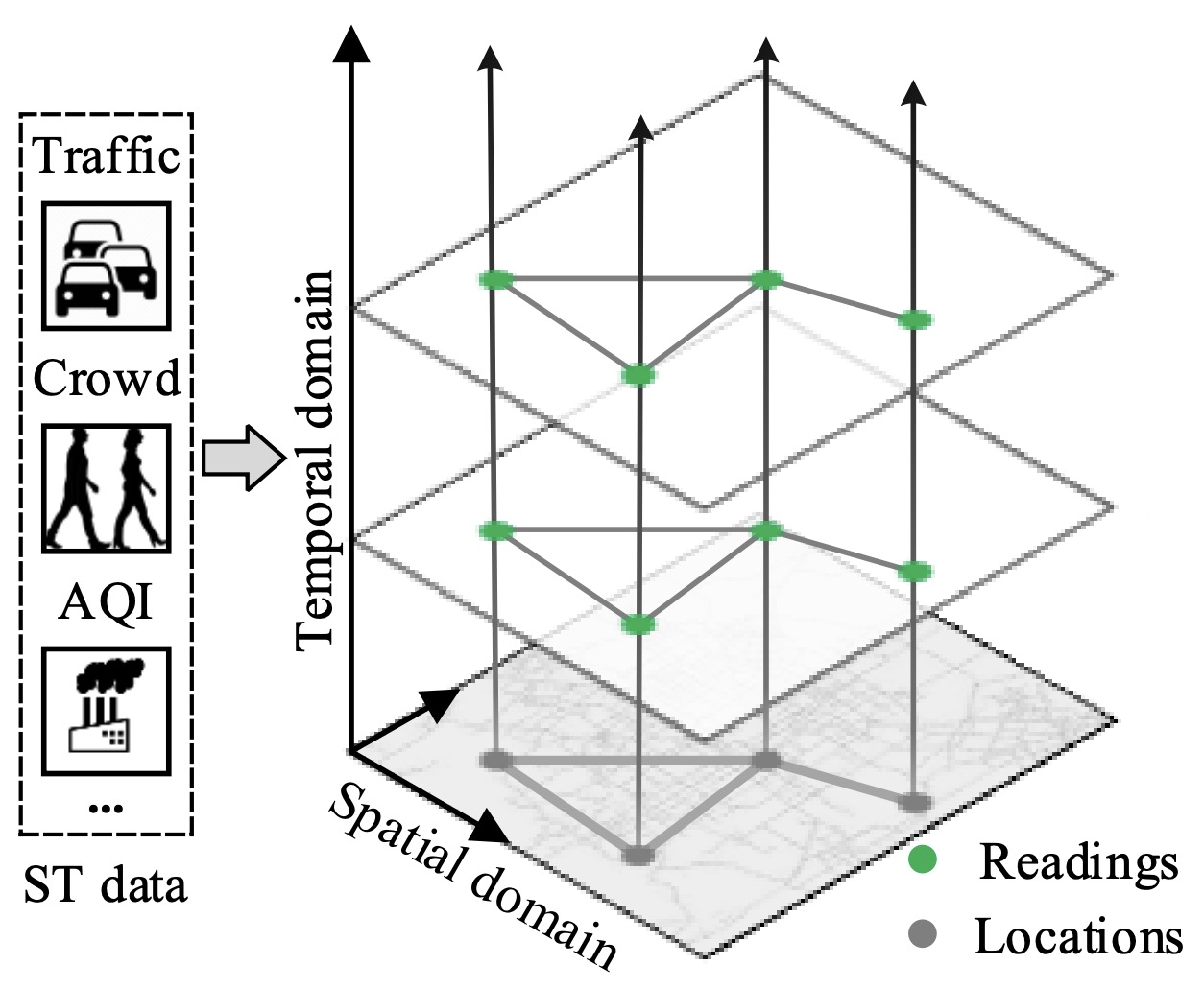
Figure 1: ST data and the related ST graph structure in urban areas

For instance, the traffic forecasting task( Forecasting highway traffic volume(i.e., # of vehicles) ) launched by California Performance of Transportation (PeMS) is one of the most popular problems in the area of spatio-temporal processing.

For this task, a diverse set of techniques have been proposed. The most important is Neural controlled differential equations (NCDEs), which are a breakthrough concept for processing sequential data.

In this paper, the author presents the method of spatio-temporal graph neural controlled differential equation (STG-NCDE). They extend the concept and design two NCDEs: one for the temporal processing and the other for the spatial processing. After that, they combine them into a single framework.

2. Motivation

It has not been studied yet how to combine the NCDE technology (i.e., temporal processing(because NCDE technology is good at time-series tasks)) and the graph convolutional processing technology (i.e., spatial processing(because graph is good at constructing position and distance)) to solve the spatio-temporal forecasting problem.

3. Proposed Method

Time-series of graphs:

\[\{\mathcal{G}_{t_i} \overset{\text{def}}{=} (\mathcal{V},\mathcal{\varepsilon},\boldsymbol{F}_i,t_i)\}_{i=0}^N ...(1)\]

where $\mathcal{V}$ is a ﬁxed set of nodes, $\mathcal{\varepsilon}$ is a fixed set of edges, $t_i$ is a time-point when $\mathcal{G}_{t_i}$ is observed, and $\boldsymbol{F}_i \in \mathbb{R}^{\vert \mathcal{V} \vert \times D}$ is a feature matrix at time $t_i$ which contains $D$-dimensional input features of the nodes, the spatio-temporal forecasting is to predict $\hat{\boldsymbol{F}} \in \mathbb{R}^{\vert \mathcal{V} \vert \times S \times M}$

For example, when we predict the trafﬁc volume for each location of a road network for the next $S$ timepoints (or horizons) given past $N + 1$ historical traffic patterns, where $\vert\mathcal{V}\vert$ is the number of locations to predict and $M = 1$ because the volume is a scalar(i.e., # of vehicles)

Here is the NCDEs, which are considered as a continuous analogue to recurrent neural networks (RNNs), can be written as follows:

\[\begin{split} z(T) &=z(0)+\int_0^Tf(z(t);\theta_f)dX(t) \\ &=z(0)+\int_0^Tf(z(t);\theta_f)\frac{dX(t)}{dt}dt ...(2) \end{split}\]

where $X$ is a continuous path taking values in a Banach space. The entire trajectory of $z(t)$ is controlled over time by the path $X$. The path $X$ is created from ${(t_i,x_i)}_{i=0}^N$ by an interpolation algorithm.

3.1 Overall design

Pre-processing and main processing steps as follows:

Its pre-processing step is to create a continuous path $X^{(v)}$ for each node $v$, where $1 \leq v \leq \vert\nu\vert$, from ${F_i^{(v)}}_{i=0}^N$. $F_i^{(v)} \in \mathbb{R}^D$ means the $v$-th row of $F_i$, and $F_i^{(v)}$ stands for the time-series of the input features of $v$.
The above pre-processing step happens before training their model. Then, their main step, which combines a GCN and an NCDE technologies, calculates the last hidden vector for each node $v$, denoted $z^{(v)}(T)$.
After that, they have an output layer to predict $\hat{y}^{(v)} \in \mathbb{R}^{S \times M}$ for each node v. After collecting those predictions for all nodes in $\nu$, they have the prediction matrix $\hat{Y} \in \mathbb{R}^{\vert\nu\vert \times S \times M}$.

3.2 Graph neural controlled differential equations (STG-NCDE)

Temporal processing

The first NCDE for the temporal processing can be written as follows:
\[h^{(v)}(T) = h^{(v)}(0) + \int_0^Tf(h^{(v)}(t);\theta_f)\frac{dX^{(v)}(t)}{dt}dt ...(3)\]
where $h^{(v)}(t)$ is a hidden trajectory (over time $t \in [0,T])$ of the temporal information of node $v$.

Eq. (3) can be equivalently rewritten as follows using the matrix notation:
\[H(T) = H(0) + \int_0^Tf(H(T);\theta_f)\frac{dX(t)}{dt}dt ...(4)\]
where $X(t)$ is a matrix whose $v$-th row is $X^{(v)}$. The CDE function $f$ separately processes each row in $H(t)$.
Spatial processing

After that, the second NCDE starts for its spatial processing as follows:
\[Z(T) = Z(0) + \int_0^Tg(Z(t);\theta_g)\frac{dH(t)}{dt}dt ...(5)\]
where the hidden trajectory $Z(t)$ is controlled by $H(t)$ which is created by the temporal processing.

After combining Eqs. (4) and (5), they have the following single equation which incorporates both the temporal and the spatial processing:
\[Z(T) = Z(0) + \int_0^Tg(Z(t);\theta_g)f(H(t);\theta_f)\frac{dX(t)}{dt}dt ...(6)\]
where $Z(t) \in \mathbb{R}^{\vert\nu\vert \times dim(z^{(v)})}$ is a matrix created after stacking the hidden trajectory $z^{(v)}$ for all $v$.

4. Experimental Evidence

Datasets

The datasets are collected by the Caltrans Performance Measurement System (PeMS) in real time every 30 seconds. The traffic data are aggregated into every 5-minute interval from the raw data. The system has more than 39,000 detectors deployed on the highway in the major metropolitan areas in California. Geographic information about the sensor stations are recorded in the datasets. There are three kinds of traffic measurements considered in our experiments, including total flow, average speed, and average occupancy.

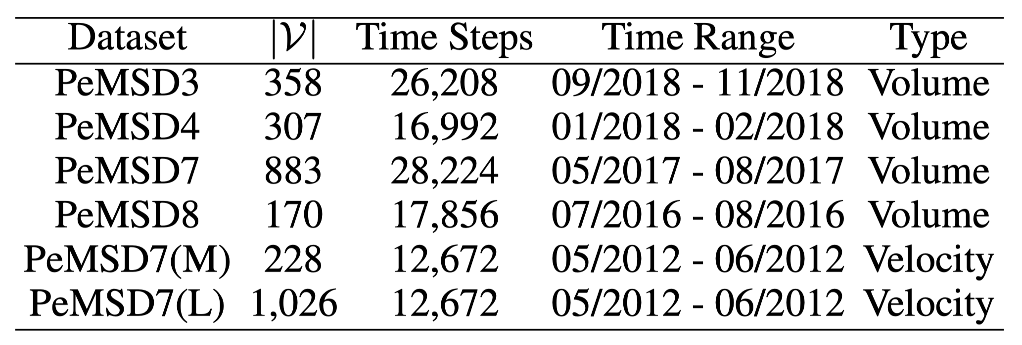
Table 1: Datasets list in this experinment

PeMSD4 Dataset Example:

distance.csv file:

from	to	cost
73	5	352.6
5	154	347.2
154	263	392.9
263	56	440.8
56	96	374.6

pems04.npz file using 307 detectors(nodes), from Jan to Feb in 2018, also contains 3 features: flow, occupy, speed. The shape is (sequence_length, num_of_vertices, num_of_features).

Baselines(parts)
- HA (Hamilton 2020) uses the average value of the last 12 times slices to predict the next value.
- ARIMA is a statistical model of time series analysis.
- VAR (Hamilton 2020) is a time series model that captures spatial correlations among all trafﬁc series.
- TCN (Bai, Kolter, and Koltun 2018) consists of a stack of causal convolutional layers with exponentially enlarged dilation factors.
- FC-LSTM (Sutskever, Vinyals, and Le 2014) is LSTM with fully connected hidden unit.
- GRU-ED (Cho et al. 2014) is an GRU-based baseline and utilize the encoder-decoder framework for multi-step time series prediction.
- DSANet (Huang et al. 2019) is a correlated time series prediction model using CNN networks and self-attention mechanism for spatial correlations.
Results

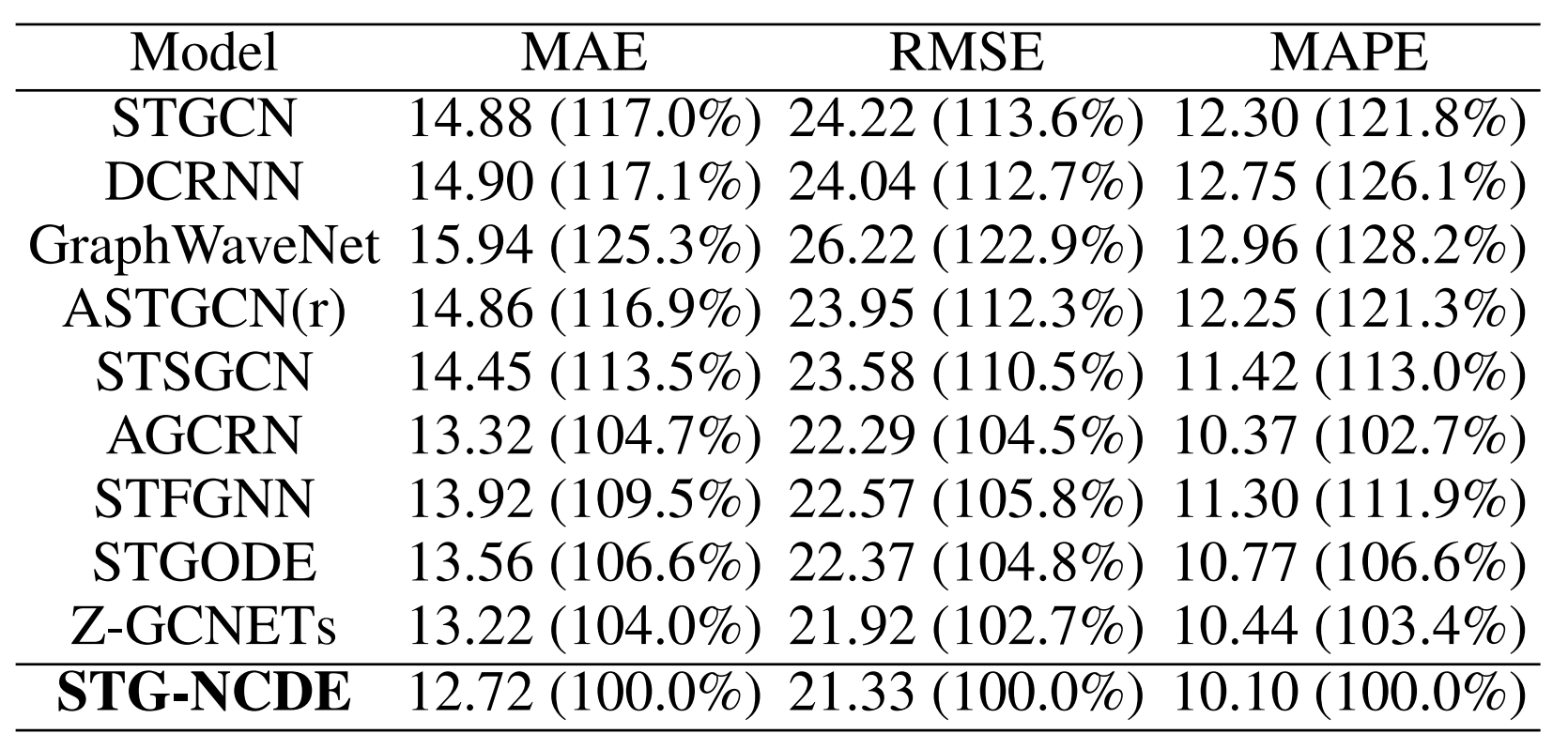
Table 2: The average error of some selected highly performing models across all the six datasets. Inside the parentheses, it shows the others performance relative to STG-NCDE.

Overall, STG-NCDE, clearly marks the best average accuracy as summarized in Table 2. For instance, STGCN shows an MAE that is 17.0% worse than that of STG-NCDE. All existing methods show worse errors in all metrics than STG-NCDE (by large margins for many baselines).

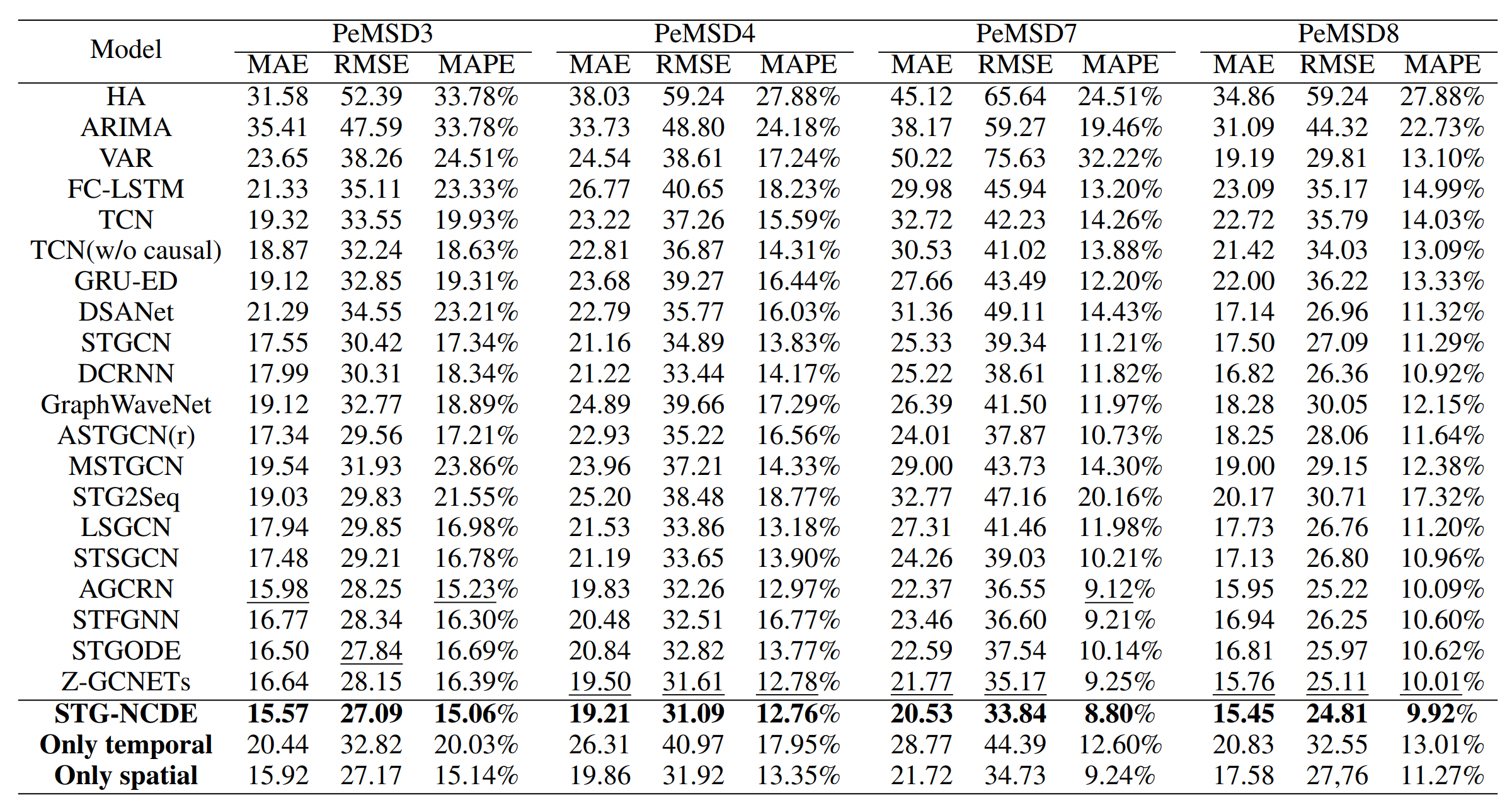
Table 3: Forecasting error on PeMSD3, PeMSD4, PeMSD7 and PeMSD8

For each dataset. STG-NCDE shows the best accuracy in all cases, followed by Z-GCNETs, AGCRN, STGODE and so on in Table 3. For instance, STGODE shows reasonably low errors in many cases, e.g., an RMSE of 27.84 in PeMSD3 by STGODE, which is the second best result vs. 27.09 by STG-NCDE. However, it is outperformed by AGCRN and Z-GCNETs for PeMSD7. Only STG-NCDE, shows reliable predictions in all cases.

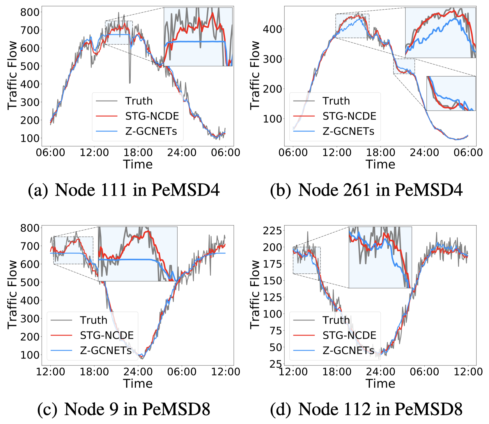
Figure 2: Trafﬁc forecasting visualization.

We can see from Fig. 2 that node 111 and 261 (resp. Node 9 and 112) are two of the highest trafﬁc areas in PeMSD4 (resp. PeMSD8). STG-NCDE shows much more accurate predictions. For example, as highlighted with boxes, STG-NCDE signiﬁcantly outperforms Z-GCNETs for the highlighted timepoints for Node 111 in PeMSD4 and Node 9 in PeMSD8 where the prediction curves of Z-GCNETs are straight which shows nonsensical predictions.

5. Conclusion

They presented a spatio-temporal NCDEs model to perform traffic forecasting: one for temporal processing and the other for spatial processing.

In their experiments with 6 datasets and 20 baselines, their method clearly shows the best overall accuracy.

In addition, their model can perform irregular traffic forecasting where some input observations can be missing, which is a practical problem setting but not actively considered by existing methods.

6. Paper Evaluation

The innovation in this paper is to propose the combination of graph convolutional network and NCDEs.

But, you need to be familiar with the two basic topics of controlled differential equations and graphs to understand more deeply. Because there is no more detailed introduction to them here. Actually, there are some parts I can’t fully understand.

In the process of converting dynamic graphs into time series, each point is converted into a sequence, and then processing is performed on each sequence. We can see that this approach results in invalid data storage. Because the graph structure will have many intersection nodes, this will cause the storage of time series to have redundancy.

Moreover, the paper involves a large number of descriptions of partial differential equations, and there is not much content that is obviously useful.

Author Information

Authors: Jeongwhan Choi, Hwangyong Choi, Jeehyun Hwang, Noseong Park

Affiliation: Yonsei University, Seoul, South Korea

Comments: Accepted by AAAI Conference on ArtiAcial Intelligence pp.6367-6374 (2022)

Cite As: https://doi.org/10.48550/arXiv.2112.03558

7. Reference & Additional materials

Github Implementation: https://github.com/jeongwhanchoi/STG-NCDE
Datasets Used: https://paperswithcode.com/dataset/pemsd8