[ICLR 2021] Dataset Condensation with Gradient Matching
Dataset Condensation with Gradient Matching
1. Introduction
Computer Vision, NLP, 음성인식 등의 분야에서 large-scale 데이터셋을 사용하는 것이 당연시되고 있다. 그러나 거대한 데이터셋을 사용하는 것은 데이터 보관 비용 및 전처리 비용이 매우 크다. 따라서 data-effiency를 발전시키는 것이 매우 중요한 분야로 자리잡기 시작하였다.
Dataset Condensaton 이전에는 coreset methods들이 활용되었다. Coreset Methods란, 거대한 데이터셋에서 데이터셋의 특성과 분포 등을 가지고 있는 작은 subset을 만드는 data selection 기법이다. 다음은 대표적인 coreset methods들이다.
- Random: 거대한 데이터셋에서 임의로 데이터를 추출하는 기법이다.
- Herding: cluster center, 즉 데이터셋의 평균이라고 추정되는 데이터를 선택하는 기법이다.
- K-Center: 데이터셋에 여러 개의 군집이 있을 때, 각 군집의 중심에 해당하는 데이터를 추출하는 기법이다. 각 군집의 중심과 군집에서 가장 멀리 떨어져있는 데이터 사이의 거리를 최소화시키는 방식으로 군집을 파악하고, 각 군집의 center point에서 데이터를 선택하게 된다.F
- forgetting: 데이터셋을 train 시킬 때, 정보가 잘 담겨있지 않아 잘 forget되는 데이터는 선택되지 않고, 정보가 많이 담겨있어 train에 용이하도록 하는 데이터를 선택하는 기법이다.
그러나 이러한 기법들은 heuristics에 의존하기 때문에, 빠르고 효율적으로 data selection이 이루어질 순 있지만 이것이 image classification 과 같은 downstream task의 최선의 solution이 아닐 수 있다. 또 데이터셋을 대표하는 subset을 만들기 때문에, 모델의 학습 성능 측면에서 최선의 solution이 아닐 수 있다는 한계점이 있다.
또 dataset synthetic method로 Dataset Distillation이 있다. Dataset distillation은 전체 training dataset에 있는 정보를 요약하여 작은 수의 synthetic training images를 만드는 기법이다. synthetic dataset은 training loss를 원본 training dataset을 기준으로 최소화시키며 학습된다. 이러한 합성 데이터는 downstream task에 최적화되어 있으며, 이미지의 모양은 크게 중요하지 않다.
Dataset Distillation과 마찬가지로 Dataset Condensation은 small sythetic images로 훈련된 모델로 최고의 일반화 성능을 얻는 것이 목표이다. Dataset Condensation의 목표를 세 가지로 정리하자면 다음과 같다.
- 커다란 이미지 분류 데이터셋을 작은 synthetic 데이터셋으로 만들어야 한다.
- synthetic 데이터셋에 이미지 분류 모델을 학습시켜 어느 정도의 성능을 내서, 추후에도 이 모델을 사용할 수 있게 되어야 한다.
- 하나의 synthetic image set으로 다양한 neural network architecture에 train시킬 수 있도록 해야 한다.
특히 이 논문에서는 Gradient Matching기법을 활용하여 dataset condensation을 진행하였는데, original dataset을 학습시킨 모델의 parameter와 condensed dataset을 학습시킨 모델의 parameter의 차이를 minimize하는 것이 dataset condensation의 목표이다. 두 개의 모델 성능은 비슷하게 될 것이며, gradients 또한 비슷하게 생성 될 것이다. 또 gradient matching기법으로 생성된 condensed dataset만을 활용하여 새로운 network를 학습시킬 때, computational load가 현저히 줄어들 것이다.
2. Method
2.1 Basic Settings
Large original dataset:
- 총 $\lvert \tau \rvert$개의 이미지들로 구성되어 있다.
- 각 이미지들은 $\tau = { (x_ {i}, y_ {i}) }\vert_ {i=1}^{\vert\tau\vert}$ $\text{ where } x \in X \subset \mathbb{R^{d}} \text{ and } y \in {0, \ldots, C-1}$ 로 표현되며, 여기서 C는 class의 개수를 말한다.
- 우리는 이러한 $\tau$를 미분 가능한 함수(i.e. deep neural network)인 $\phi$를 learn하고 싶으며, 이 함수의 parameter는 $\theta$라고 표현할 수 있다.
- $x$ 이미지에 대한 라벨 예측은, $y=\phi _ \theta (x)$ 로 표현할 수 있다.
- parameter인 $\theta$를 최적화하고 싶다면, $\theta ^ \tau = \text{argmin}_ \theta \mathcal{L}^\tau(\theta)$의 식을 통해 empirical loss term을 학습데이터에 대해 최소화시키는 $\theta$를 찾아야 한다.
- 여기서 $\mathcal{L}^\tau(\theta)$ 는 $\mathcal{L}^\tau(\theta) = \frac{1}{\vert\tau\vert} \sum_ {(x,y) \in \tau} \ell(\phi_ {\theta}(x), y)$ 를 의미하며, 이 때 $\ell(\cdot,\cdot)$는 task specific loss (i.e. cross-entropy)를 의미한다.
- $\theta ^ \tau$ 는 $\mathcal{L}^\tau$ 의 minimizer이다.
- 모델 $\phi _ {\theta^{\tau}}$ 로부터 얻을 수 있는 generalizaton performance는 $P_ D$의 데이터 분포를 따를 때, $\mathbb{E}_ {x \sim P_ D} [\ell(\phi_ {\theta^\tau}(x), y)]$라고 할 수 있다.
Small synthetic dataset:
- 총 $\lvert S \rvert$개의 이미지들로 구성되어 있다.
- 각 이미지들은 $S = { (s_ {i}, y_ {i}) }\vert_ {i=1}^{\vert S \vert}$ $\text{ where } s \in \mathbb{R^{d}} \text{ and } y \in Y$ 로 표현되며, 여기서 Y는 large original dataset의 class 개수와 같은 C개의 class를 가진다.
- 데이터셋의 크기는 synthetic dataset이 original dataset보다 훨씬 작아야 하므로, $\lvert S \rvert « \lvert \tau \rvert$로 표현할 수 있다.
- Large original dataset과 유사하게, 모델 $\phi$를 학습시키기 위해 $\theta ^ S = \text{argmin}_ {\theta} \mathcal{L}^S(\theta)$를 만족하는 최적의 parameter $\theta$를 찾을 수 있다.
- 여기서 $\mathcal{L}^{S}(\theta)$ 는 $\mathcal{L}^{S}(\theta) = \frac{1}{\vert S \vert} \sum_ {(s,y) \in S} \ell(\phi_ {\theta}(s), y)$ 를 의미한다.
- 이 때 $\theta ^ S$는 $\mathcal{L}^{S}$의 minimizer이다.
- $\lvert S \rvert$ 가 $\lvert \tau \rvert$보다 훨씬 작으므로, 최적의 $\theta$를 찾는 과정이 훨씬 빠를 것이다.
-
모델 $\phi _ {\theta^S}$ 로부터 얻을 수 있는 generalizaton performance는 $P_ D$의 데이터 분포를 따를 때, 우리는 이것이 $\phi _ {\theta^\tau}$와 유사하도록 condensed set을 만들고싶다. 이를 식으로 표현하면 다음과 같다. $\mathbb{E}_ {x \sim P_ {D}} [\ell(\phi_ {\theta^{\tau}}(x), y)] \stackrel{\sim}{=} \mathbb{E}_ {x \sim P_ D} [\ell(\phi_ {\theta^{S}}(x), y)]$
- $\mathbb{E}_ {x \sim P_ {D}} [\ell(\phi_ {\theta^{\tau}}(x), y)] \stackrel{\sim}{=} \mathbb{E}_ {x \sim P_ {D}} [\ell(\phi_ {\theta^{S}}(x), y)]$ 의 식을 다르게 formulate해보면 다음과 같다.
$\min_ {S} D(\theta^{S}, \theta^{\tau}) \text{ subject to } \theta^{S}(S) = \text{argmin}_ {\theta} \mathcal{L}^{S}(\theta)$ - 이 때 $\theta^{\tau} = \text{argmin}_ \theta \mathcal{L}^{\tau}(\theta)$ 이며, $D(\cdot,\cdot)$ 는 distance function을 의미한다.
2.2 Dataset Condensation with Curriculum Gradient Matching
- Dataset Conensation with Parameter Matching의 문제점을 해결하기 위해, 해당 논문은 Dataset Condensation with Curriculum Gradient Matching 기법을 제시하였다.
- 간결한 논문 리뷰를 위해 Dataset Conensation with Parameter Matching의 문제점은 5의 Related Works에 더 자세히 설명하였다.
- 본 아이디어의 목적은 $\theta^{\tau}$와 $\theta^{S}$가 유사해야 할 뿐 만 아니라, 최적화 과정에서 $\theta^{\tau}$와 $\theta^{S}$이 유사한 path를 따라야 한다는 것이다.
- 이러한 목적을 반영하여 다음과 같은 수식을 도출하였다.
- $T$는 iteration 숫자를, $\varsigma^{\tau}$와 $\varsigma^{S}$는 $\theta^\tau$와 $\theta^S$의 최적화 steps 숫자를 의미한다.
$\min_ S \mathbb{E}_ {\theta_ 0\sim P_ {\theta_ 0}}[\sum^{T-1}_ {t=0} D(\theta^S_ t. \theta^\tau_ t)]$
$\text{subject to } \theta^S_ {t+1}(S) = \text{opt-alg}_ \theta(\mathcal{L}^S(\theta^S_ t), \varsigma^S) \text{ and } \theta^\tau_ {t+1} = \text{opt-alg}_ \theta(\mathcal{L}^\tau(\theta^\tau_ t), \varsigma^\tau)$ - 이 식은 각 iteration에서의 $\theta^S$와 $\theta^\tau$의 거리가 최소화되도록 한다.
- 이를 모든 iteration에 대해서 적용하고, 0 iteration부터 $T-1$ iteration까지 모두 합하게 되어 각 iteration마다의 세타 값들을 유사하게 맞출 수 있게 된다.
- 여기서 $S$를 적절히 업데이트하고 $D(\theta^S_ t. \theta^\tau_ t)$를 0으로 근사시키게 된다면 $\theta^S_ {t+1}$은 $\theta^\tau_ {t+1}$를 성공적으로 tracking할 수 있게 된다.
- $T$는 iteration 숫자를, $\varsigma^{\tau}$와 $\varsigma^{S}$는 $\theta^\tau$와 $\theta^S$의 최적화 steps 숫자를 의미한다.
- 또, 다음 iteration으로의 $\theta$ update rule은 다음과 같다.
- $\eta_ \theta$는 learning rate를 의미한다.
$\theta^S_ {t+1} \leftarrow \theta^S_ t - \eta_ \theta \nabla_ \theta \mathcal{L}^S(\theta^S_ t) \quad \text{and} \quad \theta^\tau_ {t+1} \leftarrow \theta^\tau_ t - \eta_ \theta \nabla_ \theta \mathcal{L}^\tau(\theta^T_ t)$
- $\eta_ \theta$는 learning rate를 의미한다.
- 여기서 $D(\theta^S_ t. \theta^\tau_ t)\approx 0$이기 때문에, 위의 minimization 식을 다음과 같이 쓸 수 있다.
- $\theta^S_ t$를 $\theta^\tau_ t$로, $\theta^S$를 $\theta$로 대체할 수 있다.
$\min_ {S} \mathbb{E}_ {\theta_ 0 \sim P_ {\theta_ 0}} \left[ \sum_ {t=0}^{T-1} D\left(\nabla_ {\theta} \mathcal{L}^S(\theta_ t), \nabla_ {\theta} \mathcal{L}^\tau(\theta_ t)\right) \right]$
- $\theta^S_ t$를 $\theta^\tau_ t$로, $\theta^S$를 $\theta$로 대체할 수 있다.
Algorithm
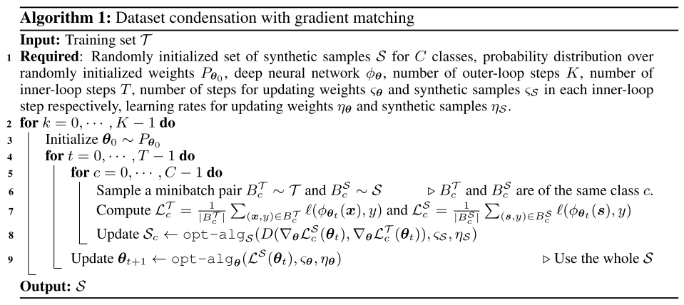
- Input으로 large original dataset인 $\tau$를 넣게 된다.
- Outer-loop steps $K$를 정하고, $K$번의 outer-loop를 돌리게 된다. 즉 $K$번의 실험을 통해 총 $K$개의 synthetic set을 만들게 된다.
- 또 $\theta_ 0$가 분포 $P_ {\theta_ 0}$를 따르도록 initialize한다.
- Inner-look steps $T$를 정하고, $T$번의 inner-loop를 돌리게 된다. 즉 하나의 synthetic set을 $T$번 update시킨다.
- Synthetic samples $S$는 $C$개의 class를 가지고 있다.
- 각 $\tau$와 $S$에 대하여 minibatch pair $B_ c^\tau$와 $B_ c^S$를 생성한다.
- 위에서 언급하였던 수식대로 loss함수인 $\mathcal{L}_ c^\tau$와 $\mathcal{L}_ c^S$를 계산한다.
- 또 위에서 언급하였던 수식대로 $S_ c$를 update한다.
- $\theta_ {t+1}$을 $\text{opt-alg}$ 알고리즘에 맞춰 update해준다.
- 이렇게 된다면 output으로 synthethized 된 subset $S$가 도출되게 된다.
3. Experiment
3.1 Dataset Condendation
Comparison to coreset methods
- Dataset
- MNIST, SVHN, FashionMNIST, CIFAR10의 총 4가지 benchmark datasets를 사용하였다.
- Architectures
- MLP, ConvNet, LeNet, AlexNet, VGG-11, ResNet-18의 총 6가지 standard deep network architectures를 사용하였다.
- Experiment Settings
- learning the condensed images 파트와 training classifiers from scratch 파트 모두 Convnet을 사용하였다.
- 1,10,50 images per class(IPC)로 실험을 진행하였다.
- 각 methods는 총 5번 실행되었다. 즉 synthetic set는 총 5개가 생성되었다.
- 각 synthetic set들은 20개의 randomlt initialized된 ConvNet 모델에 평가되었다. Model의 accuracy가 평가 대상이다.
- 5개 set에 20번의 evaluation, 총 100개의 evaluation이 진행되었고 이의 평균과 분산이 계산되었다.
- Baselines
- 4가지의 coreset methods(random, herding, K-Center, forgetting)를 사용하였다.
- Results
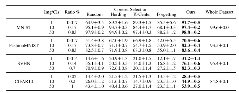
- MNIST, FashionMNIST, SVHN, CIFAR10 데이터셋에서 Dataset Condensation을 사용하여 Coreset Methods와 분류 정확도를 비교한 결과, 모든 baseline models를 크게 앞서는 성능을 보였다.
- 전체 데이터셋으로 훈련한 결과를 upper-bound 성능으로 기준삼았다.
- MNIST에서는 class당 50개의 이미지를 사용했을 때 98.8%의 성능을 달성하여, 클래스당 6000개의 훈련 이미지를 사용한 upper-bound 성능인 99.6%와 비슷한 결과를 보였다.
- FashionMNIST에서도 높은 성능을 보였지만, SVHN과 CIFAR10에서는 다양한 전경과 배경이 포함된 이미지로 인해 upper-bound와의 정확도 차이가 더 컸다.
- Random selection은 10개와 50개 이미지 당 클래스에서 다른 coreset methods와 비교해 비교적 높은 성능을 보였으며, herding 방법이 가장 좋은 coreset method로 보여졌다.
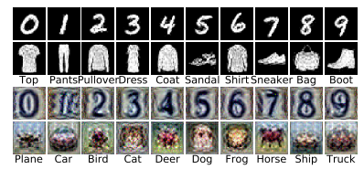
- IPC 1의 설정에서 dataset condensation으로 생성된 압축 이미지를 시각화했을 때, 각 클래스의 “프로토타입”처럼 보이며 해석 가능했다.
Comparison to DD
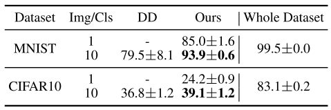
- Dataset Distillation의 실험 설정과 동일한 아키텍처를 사용하여 LeNet과 AlexCifarNet에서 MNIST와 CIFAR10 데이터셋을 사용해 실험을 수행하였고, 결과는 위의 표와 같았다.
- MNIST와 CIFAR10 두 벤치마크 데이터셋에서 더 높은 성능을 보였다. 특히 IPC가 1일 때의 dataset condensation 정확도가 IPC가 10일 때의 dataset distillation 정확도보다 5% 더 높음을 보였다.
- 여러 번 실험을 진행하였을 때, 결과들은 표준편차이 dataset condensation에서는 일관되게 나타났으며, 특히 MNIST ipc10에서 표준 편차는 0.6%에 불과했다. 반면, dataset distillation의 성능은 실험마다 크게 달라졌으며(8.1%의 표준 편차), 더 높은 변동성을 보였다.
- dataset condensation은 dataset distillation보다 CIFAR10 실험에서 2배 빠른 훈련 속도를 보였고, 메모리 사용량도 50% 줄일 수 있었다.
Cross-architecture generalization
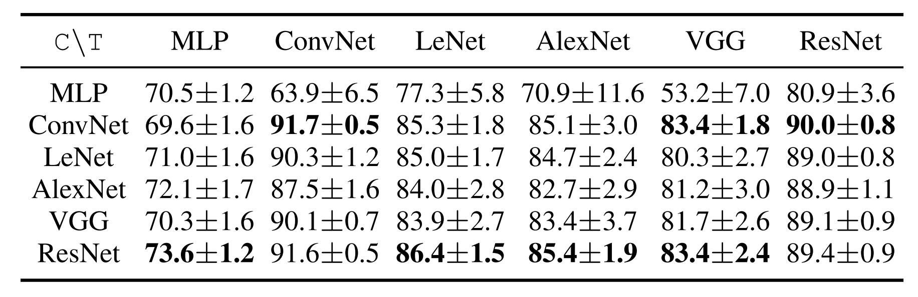
- Dataset condensation의 장점 중 하나는 하나의 아키텍처에서 학습된 압축 이미지를 다른 아직 보지 못한 아키텍처의 훈련에 사용할 수 있다는 것이다.
- 다양한 네트워크(MLP, ConvNet, LeNet, AlexNet, VGG-11, ResNet-18)를 통해 MNIST 데이터셋의 ipc1 합성 데이터셋을 학습하고, 이를 각 네트워크에 별도로 적용하여 MNIST 테스트 세트에서 분류 정확도를 평가하였다.
- 그 결과 특히 convolutional architecture로 훈련된 condensed set이 높은 성능을 보이며, 이는 다양한 architecture에 걸쳐 범용성이 있음을 보여준다.
- MLP로 생성된 이미지는 convolutional architecture training에는 적합하지 않았으나, convolutional architecture로 생성된 이미지를 사용했을 때는 더 나은 성능을 보였다.
- 가장 좋은 결과는 대부분 ResNet으로 생성된 이미지와 ConvNet 또는 ResNet을 classifier로 사용했을 때였다.
Number of condensed images
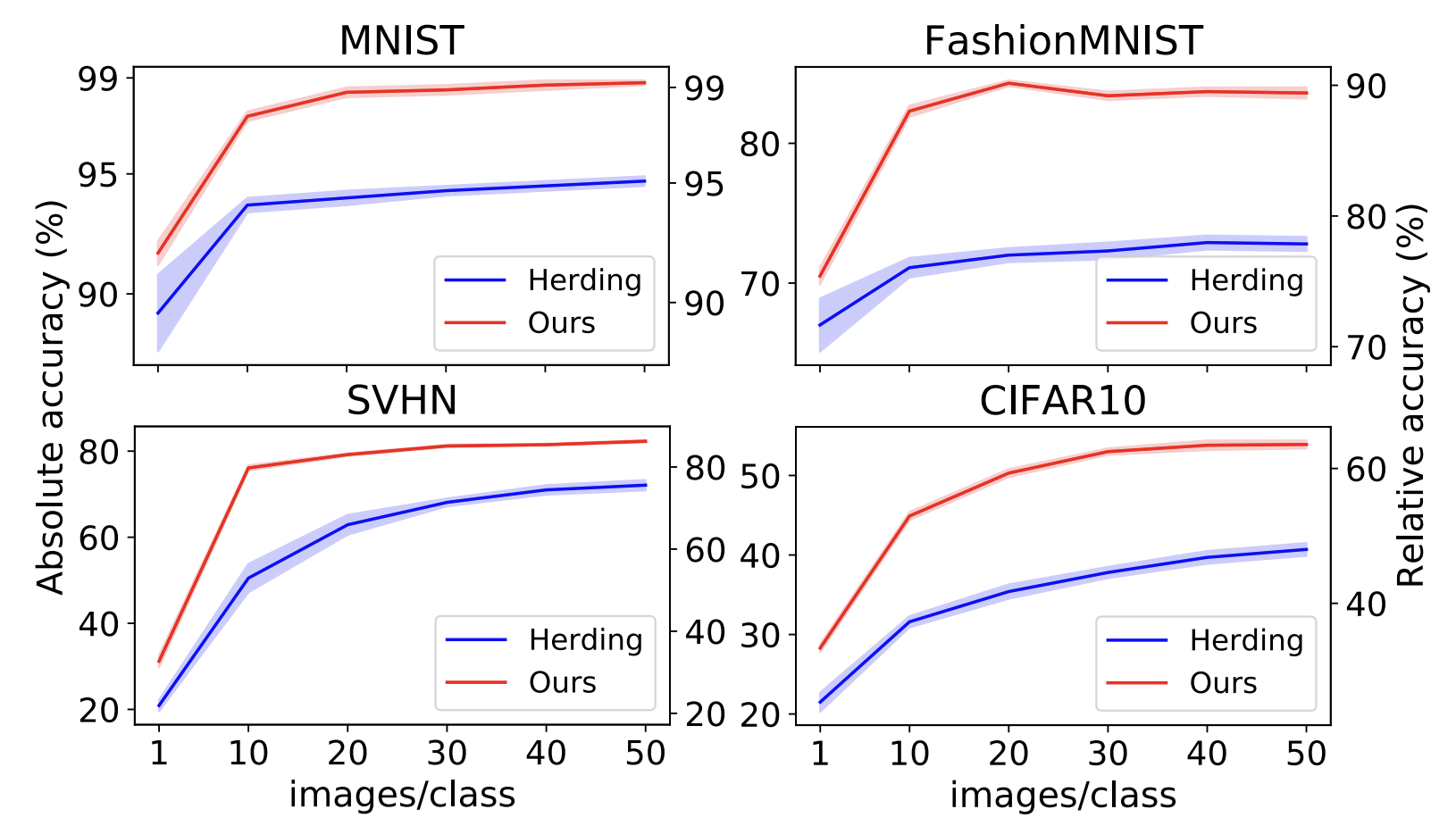
- MNIST, FashionMNIST, SVHN, CIFAR10를 training dataset으로 사용하여 ConvNet을 훈련시키는 실험을 수행하였다.
- ipc를 늘릴수록 모든 벤치마크에서 정확도가 향상되며, 특히 MNIST와 FashionMNIST에서는 상한선(upper-bound) 성능과의 격차가 줄어들었다.
- SVHN과 CIFAR10에서는 ipc가 크더라도 여전히 upper-bound와의 격차가 크다.
- 기존 코어셋 방식인 Herding 방법보다 모든 경우에서 큰 차이로 우수한 성능을 보인다.
Activation, normalization & pooling
- Activation function과 pooling and nomalization function이 dataset condensation에 미치는 영향을 살펴보기 위해 실험을 수행하였다.
- Activation function으로는 sigmoid, ReLU, leaky ReLU를, pooling and nomalization function으로는 max pooling, average pooling, batch normalization, group normalization, layer normalization, instance normalization을 평가하였다.
- 그 결과, leaky ReLU는 ReLU보다, average pooling은 max pooling보다 더 나은 압축 이미지 학습을 가능하게 한다.
- 이는 leaky ReLU와 average pooling이 더 조밀한 그래디언트 흐름을 제공하기 때문이다.
- 또 작은 condensed set으로 훈련된 네트워크에서 instance normalization이 다른 정규화 방법들보다 더 좋은 분류 성능을 보였다.
3.2 Applications
Continual Learning
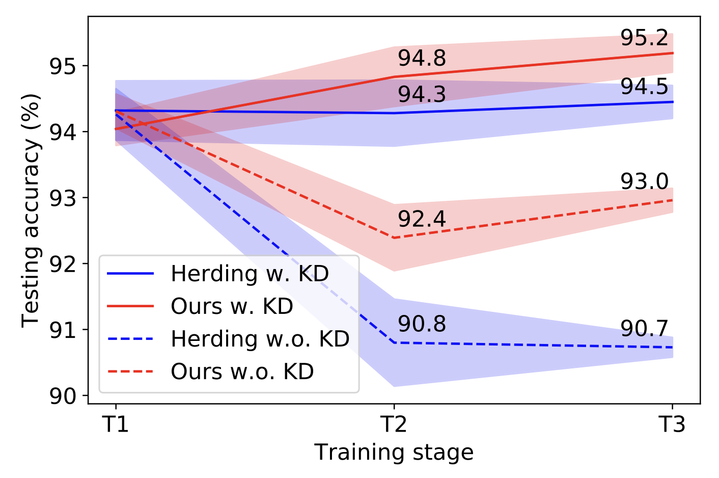
- Dataset condensation을 continual learning 시나리오에서 적용하여, 새로운 task를 점진적으로 학습하며 기존 task의 성능을 유지하는 것이 목표이다.
- 논문의 모델은 E2E 방법을 사용였으며, 제한된 예산의 rehearsal 메모리(ipc 10)와 knowledge distillation(KD)을 사용하여 이전 예측에 대한 네트워크의 출력을 규제하였다.
- Sample selection mechanism은 기존의 herding 방법 대신에 dataset condensation을 통해 condensed dataset을 생성하여 메모리에 저장하는 방식으로 대체하였다.
- Digital recognition dataset인 SVHN, MNIST, USPS을 사용한 task-incremental learning problem에서 모델을 평가하였다.
- KD regularization의 사용 여부에 따라 E2E 방법과 dataset condensation을 비교하였다. 실험은 3단계의 incremental training stages(SVHN→MNIST→USPS)을 포함하고 각 단계 후 이전 및 현재 task의 테스트 세트를 평균하여 정확도를 계산하였다.
- 그 결과, condensed set이 herding으로 샘플링된 이미지보다 데이터 효율이 높으며, KD가 사용되지 않을 때 (T3에서 2.3% 차이) 특히 더 높은 성능을 보였다.
Neural Architecture Search
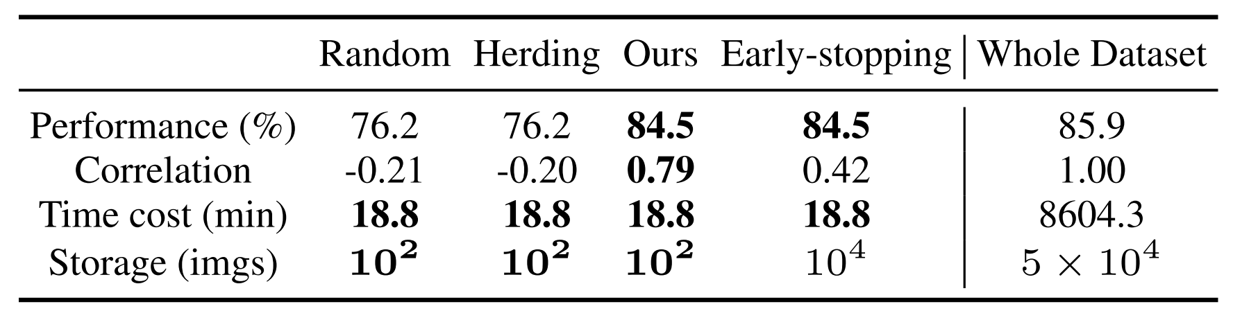
- Neural Architecture Search (NAS) 실험을 통해 condensed image를 활용하여 다양한 네트워크를 효율적으로 훈련시켜 최적의 네트워크를 식별할 수 있는지를 검증하였다.
- 훈련은 CIFAR10 데이터셋에 대해서 진행되었다.
- 하이퍼파라미터(W, N, A, P, D)를 변형시켜 720개의 ConvNet 아키텍처를 구성하였고, ipc 10인 3개의 small proxy dataset(Random sampling, Herding, Dataset Condensation)에서 100 epochs 동안 훈련하였다.
- 또 전체 데이터셋 훈련에 early-stopping를 한 성능과 비교분석을 하였는데, 이 때 small proxy dataset에 필요한 훈련 계산량만을 사용하도록 early-stopping을 시켰다.
- 실험 결과로, dataset condensation을 활용하였을 때 최고 성능 모델의 평균 테스트 성능이 84.5%로 가장 높았다.
- 또 상관계수 0.79로 proxy 데이터셋과 전체 데이터셋 훈련 간 높은 성능 상관관계를 보였다.
- 반면에 early-stopping을 활용한 상위 10개 모델의 rank correlation (0.42)은 dataset condensation을 활용한 상위 10개 모델의 rank correlation (0.79)보다 현저히 작았다.
- NVIDIA GTX1080-Ti GPU에서 720개 아키텍처의 훈련 시간이 8604.3분에서 18.8분으로 대폭 감소하였다.
- 훈련 이미지의 저장 공간은 5 × 10^4개에서 1 × 10^2개로 줄어들었다.
4. Conclusion
해당 논문은 정보를 많이 담은 소수의 합성 이미지를 만들 수 있는 dataset condensation 방법을 제안한다.이 기법으로 만들어진 condensed dataset은 기존 이미지나 이전 방법들로 생성된 이미지들보다 데이터 효율성이 높으며, 다양한 딥러닝 아키텍처에 종속되지 않아 여러 네트워크 훈련에 사용될 수 있다. Condensed dataset은 메모리 사용량을 줄이고, continual learning 및 neural architecture search에서 다수의 네트워크를 효율적으로 훈련하는 데 중요한 역할을 한다. 추가적인 발전 방향으로는, 더 다양하고 도전적인 데이터셋인 ImageNet에서 condensed dataset의 활용 가능성 탐구가 있다.
Author Information
- Bo Zhao, Konda Reddy Mopuri, Hakan Bilen
- School of Informatics, The University of Edinburgh
- Computer Vision and Pattern Recognition
5. Reference & Additional materials
- Github Implementation
- Bo Zhao, Konda Reddy Mopuri, and Hakan Bilen. Dataset condensation with gradient matching. ICLR, 1(2):3, 2021.
- Tongzhou Wang, Jun-Yan Zhu, Antonio Torralba, and Alexei A Efros. Dataset distillation. arXiv preprint arXiv:1811.10959, 2018.
Related Works
Methodoldgy for Dataset Conensation with Parameter Matching
- 2.1에서 언급하였던 $\mathbb{E}_ {x \sim P_ {D}} [\ell(\phi_ {\theta^{\tau}}(x), y)] \stackrel{\sim}{=} \mathbb{E}_ {x \sim P_ {D}} [\ell(\phi_ {\theta^{S}}(x), y)]$ 의 식을 다르게 formulate해보면 다음과 같다.
$\min_ {S} D(\theta^{S}, \theta^{\tau}) \text{ subject to } \theta^{S}(S) = \text{argmin}_ {\theta} \mathcal{L}^{S}(\theta)$ - 이 때 $\theta^{\tau} = \text{argmin}_ \theta \mathcal{L}^{\tau}(\theta)$ 이며, $D(\cdot,\cdot)$ 는 distance function을 의미한다.
- 현실에서 $\theta^{\tau}$는 initial value인 $\theta_ {0}$에 의해 결정되게 된다.
- 다만, 이 식에서는 initialization $\theta_ {0}$에만 해당하는 하나의 모델 $\phi_ {\theta^{\tau}}$에 대해서만 최적의 synthetic images만 얻을 수 있게 된다.
- 따라서 저자는 이를 방지하기 위해 random initialization의 분포 $P_ {\theta_ {0}}$를 정의하였다.
- 이를 활용하여 위의 distance function을 활용한 minimization 식을 다음과 같이 바꿀 수 있다.
$\min_ S E_ {\theta_ {0} \sim P_ {\theta_ {0}}} [D(\theta^{S}(\theta_ {0}), \theta^{\tau}(\theta_ {0}))] \text{ subject to } \theta^{S}(S) = \text{argmin}_ {\theta} \mathcal{L}^{S}(\theta(\theta_ {0}))$
- 여기서 $\theta^{\tau} = \text{argmin}_ {\theta} \mathcal{L}^{\tau}(\theta(\theta_ {0}))$이다.
- 앞으로 간결화를 위해 $\theta^{\tau}(\theta_ {0})$는 $\theta^{\tau}$로, $\theta^ {S}(\theta_ {0})$는 $\theta^{S}$로 표현할 예정이다.
- inner loop operation인 $\theta^{S}(S) = \text{argmin}_ {\theta} \mathcal{L}^{S}(\theta)$는 large-scale 모델에서 컴퓨팅적 비용이 매우 높기 때문에, 이를 back-optimization approach를 활용하였다.
- 따라서 $\theta^{S}$를 다음과 같이 재정의하였다. $\theta^{S}(S) = \text{opt-alg}_ {\theta}(\mathcal{L^{S}(\theta), \varsigma})$
- 여기서 $\text{opt-alg}$란 정해진 시행 횟수 $\varsigma$에서의 특정 최적화 과정을 말한다.
- 그러나 이러한 과정을 통한 synthetic dataset 합성은 두 가지 문제점이 있다.
- $\theta^{\tau}$와 $\theta^S$사이의 거리가 parameter space에서 너무 클 수 있다.
- $\text{opt-alg}$를 사용하는 것은 속도와 정확도 사이의 trade-off를 유발하게 된다.