[RecSys 2023] STRec: Sparse Transformer for Sequential Recommendations
Title
STRec: Sparse Transformer for Sequential Recommendations
1. Problem Definition
Transformer 구조가 급속도로 발전함에 따라 researcher들은 SRS(sequential recommender systems)에서 Transformer 구조를 적용하고 이전 SRS model들에 비해 SRS task에 대하여 발전된 성능을 나타내는 model을 제시하고 있다.
이 논문에서 user-item interaction history는 다음과 같이 정의된다.
$\begin{align}S = {(v_ 1, t_ 1), \ldots, (v_ n, t_ n ), \ldots, (v_ N, t_ N )} \end{align}$
여기서 $v_ n \in V$는 timestamp $t_ n$에서 sequence $S$의 $n$번째 interacted item이고 $N$은 sequence의 최대 길이이다.
단순화를 위해 user 및 실제 길이에 대한 표기는 생략되었고 interacted timestamp $t_ n$을 고려한다.
SRS는 제공된 길이가 $N$인 interaction sequence ${(v_ 1, t_ 1), \ldots, (v_ N, t_ N )}$를 활용해서 다음 interacted item $v_ {N+1}$을 예측해야 하는 문제이다.
그러나 대부분의 기존 transformer 기반 SRS model들은 모든 item-item pair 간의 attention score를 계산하는 vanilla attention mechanism을 사용하고 있다.
이 경우 중복되는 item interaction으로 인해 model 성능이 저하되고 많은 계산 시간과 메모리를 필요로 할 수 있다는 문제점이 발생한다.
2. Motivation
vanilla self-attention을 transformer 기반 SRS model에 활용하면 모든 item interaction을 scan할 수 있지만 모든 interaction을 scan할 경우 막대한 계산 시간과 메모리 비용이 발생하여 SRS 모델의 inference 효율성이 저하된다.
게다가 최적이 아닌 item interaction을 고려할 수 있어 추천 성능이 저하될 수 있다.
따라서 inference 효율성과 추천 성능을 높이기 위해 필요한 item interaction을 구별할 수 있는 효율적인 transformer 구조를 설계하는 것이 필요하다.
효율적인 Transformer 구조를 설계하기 위해 다음과 같은 노력이 이루어졌다.
- Longformer, Big Bird : sparce attention 전략을 사용하여 필수적인 token pair에 대해서만 attention score를 계산
- Linformer : low-rank approximation 방법을 사용하여 attention score 계산
- Autoformer : 시계열 예측을 위해 sequence를 분해
- FLASH : vanilla attention을 gated attention unit으로 대체
- Reformer : locality-sensitive hashing(lsh) module 적용
하지만 위의 방법들은 SR(Sequential recommendation)을 위한 목적으로 설계되지 않았기 때문에(NLP나 시계열 예측을 위한 목적으로 설계됨) SR task에 직접 적용하면 추천 성능이 저하될 수 있다.
새로운 transformer 구조 설계가 필요한 이유를 아래 Figure 1을 통해 설명하고 있다.
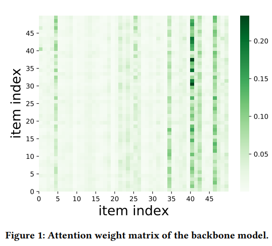
Figure 1의 Attention weight matrix를 통해 SRS task에서의 transformer 기반 model이 높은 sparsity를 보이는 것을 알 수 있다. 논문에서는 해당 sparse attention에서 보이는 low-rank phenomenon을 두 가지 측면에서 설명하고 있다.
- 극히 일부의 interaction이 output에 차이를 만든다. (heatmap column level)
- attention weight vector가 유사하고 이것이 low-rank phenomenon을 가중시킨다. (heatmap row level)
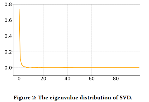
low-rank phenomenon은 attention weight matrix의 행에 대한 SVD 분해를 통해 명확히 드러난다. Figure 2를 통해 eigenvalue의 분포를 확인할 수 있다.
x축은 eigenvalue, y축은 value의 비율이다.
대부분의 eigenvalue는 상대적으로 작다. 이를 통해 low-rank matrix를 사용하여 original attention weight matrix를 근사화 할 수 있음을 알 수 있다.
이러한 현상을 바탕으로 이 논문에서는 효율성을 위해 일부 interaction 쌍만 transformer layer에서 계산하는 sparse transformer 모델(STRec)을 제안하였다.
Sparse Transformer model for sequenctial Recommendation tasks(STRec)는 cross-attention와 학습 가능한 parameter를 활용한 sampling 전략을 기반으로 한다.
3. Method
STRec은 transformer 기반 backbone model을 기반으로 구성되었다. Figure 3를 통해 STRec 모델 구조를 확인할 수 있다.
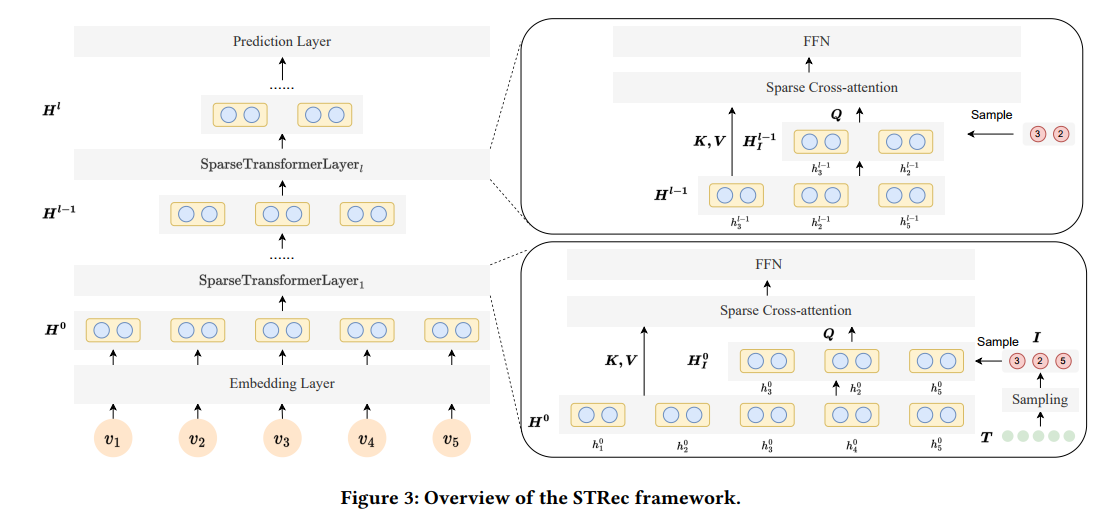
Model은 Embedding layer, 여러 Transformer layer, Prediction layer로 구성되어 있다.
Backbone model과 비교했을 때 TransformerLayer에서 차이가 있는데, 논문에서는 cross-attention과 학습 가능한 parameter를 활용한 효율적인 sampling 전략을 기반으로 하는 sparse transformer를 활용한다.
Model의 각 layer를 설명하되 이 논문의 핵심인 Cross Attention Transformer Layer와 Sampling 전략 부분을 좀 더 자세히 설명할 예정이다.
3.1 Embedding Layer
ID embedding과 positional embedding을 통합한 input item의 초기 표현을 식으로 나타내면 다음과 같다.
$ \begin{align}h_ {n}^{0} = e_ n + p_ n \end{align}$
여기서 $e_ n$은 item $v_ n$에 대한 ID embedding이고, $p_ n$은 sequence의 item index $n$에 대한 positional embedding이다. $h_ {n}^{0}$의 위 첨자 index 0는 embedding layer임을 나타낸다.
3.2 Sparse Transformer in STRec
3.2.1 Cross Attention Transformer Layer
Attention layer의 계산 비용을 줄이기 위해 vanilla self-attention을 cross-attention으로 대체하였다.
cross-attention은 input sequence를 key, value로 샘플링된 item sequence를 query로 사용한다.
sampling된 query matrix는 기존 query matrix에 비해 크게 축소되기 때문에 계산이 더 효율적이다.
$H^ {l-1}$에 대해서 cross-attention은 다음과 같은 식으로 나타낼 수 있다.
$ \begin{align} \tilde{H}^ {l-1} = Add\&Norm\left(Attention\left(H_{I}^ {l-1}, H^ {l-1}, H^ {l-1}\right) \right) \end{align}$
$\tilde{H}^ {l-1}$은 사전 정의된 $k_l$의 길이를 갖으며 sampling index $I_l$에 의해 $H_ {l-1}$에 있는 item representation이 sampling된 부분집합이다.
$\tilde{H}^ {l-1}$은 $H_{I}^ {l-1}$과 똑같은 shape를 갖는다.
FFN layer는 짧아진 $\tilde{H}^ {l-1}$를 input으로 하여 output hidden state를 만들어 낸다.
$ \begin{align} {H}^ {l} = Add\&Norm\left(FFN\left(\tilde{H}^ {l-1} \right)\right) \end{align}$
output hidden state $H^ {l}$의 길이는 여전히 $k_l$이며, $H_{I}^ {l-1}$, $\tilde{H}^ {l-1}$과 똑같은 shape를 갖는다.
vanila self-attention transformer layer와 비교했을 때 cross-attention layer는 attention과 feed-forward network 모두에서 sampled item에 대해서만 계산한다.
시간 복잡도와 공간 복잡도 모두 $O(n^ 2)$에서 $O(nk_ l)$로 감소한다.
3.2.2 Sampling strategy
Figure 1을 통해 후방 item이 SR task에서 중요할 가능성이 높음을 알 수 있다. 따라서 논문에서는 마지막 item과의 time interval을 바탕으로 학습 가능한 parameter를 사용해서 sampling 전략을 수행한다. time interval은 $T = {\tilde{t}_ i}_ {1 \le i \le N}$로 표현한다.
$ \begin{align} \tilde{t}_ {i} = t_ i - t_ N \end{align}$
$t_ i, 1 \le i \le N$은 interaction $v_ i$에 대해 기록된 timestamp이다.
첫번째 layer의 경우 MLP(Multi-layer Perceptron)을 활용해서 time interval $T$를 sampling density로 mapping한다. 무작위 샘플링을 위해 uniform distribution을 갖는 random matrix $R$ 을 추가한다. sampling index $I$는 다음과 같이 생성된다.
$ \begin{align} I_ {1} = Top_k\left(MLP(T) + R, k_ 1\right) \end{align}$ $ \begin{gather} r_ {i} \sim Uniform\left(0, 1\right) \nonumber \end{gather}$
$Top_k\left(\cdot \right)$는 내림차순으로 정렬된 index들의 set을 생성한다. $k_ 1$은 hyperparameter로서 첫번째 layer의 pre-define된 sample size이다.
이후 layer들에 대해서 sampling index를 layer별로 생성하는데는 많은 시간이 걸린다. 따라서 $MLP\left(T \right) + R$ 부분은 모든 layer에 대해 fine-tuning 및 inference 과정에서 동일하게 유지된다.
논문에서는 정렬된 index $I_ 1$를 입력하고 첫 $k_ l$개의 index를 $I_ l$로 사용한다.
$ \begin{align} I_ {l} = I_ 1\left[1: k_ l\right] \end{align}$
$ \begin{align} {H}_ {I}^ {l-1} = \left[{h}_ {I_ l \left[1\right]}^ {l-1}, \ldots, {h}_ {I_ l \left[k_ l\right]}^ {l-1} \right]
∀ 2 \le l \le L \end{align}$
$I$는 미분 가능한 방식으로 근사된(하지만 미분 가능한 방식으로 처리하기 어려운) hard decision을 생성하는 random process를 요구하는 $Top_k$ 연산 으로 인해 미분 불가능하다.
이러한 문제를 해결하기 위해 pre-train 과정에서 Gumbel-Softmax를 적용하여 sampling 과정을 attention mask $M$으로 대체한다.
여기서 $m_ {ij} \approx 0$은 $i$번째 query와 $j$번째 key 간의 attention weight가 계산되지 않았음을 의미하고 그 반대의 경우(계산된 경우)는 $m_ {ij} \approx 1$이다.
$ \begin{align} S_ {l} = Sigmoid\left(MLP\left(T\right) + R + \alpha _ l\right) ∀ 1 \le l \le L \end{align}$ $ \begin{align} S_ {0} = \left[ 1, 1, \ldots, 1\right] \end{align}$ $ \begin{align} M_ {l} = S_ {l-1} \otimes S_ {l} ∀ 1 \le l \le L \end{align}$
$\begin{gather} r_ {i} \sim Uniform\left(0, 1\right) \nonumber \end{gather}$
$MLP\left(\cdot\right)$는 normalization이 포함된 multi-layer perceptron이다.
$\alpha$는 sampling될 interaction 수(mask matrix $S_l$의 1 개수)를 제어하는데 사용된다.
$\alpha_ {l}$이 커지면 해당 layer에서 더 많은 sample이 생성된다.
layer $S_ {l}$과 그 이전 layer $S_ {l-1}$을 활용하여 attention mask matrix는 outer product $\otimes$로 계산된다.
이때 query-key pair를 뽑으면 query는 $S_ {l}$에서 나오고 key는 $S_ {l-1}$에서 나온다
attention mask $M$이 있는 미분 가능한 attention layer는 다음과 같이 표현된다.
$ \begin{align} \tilde{H}^ {l-1} = Add\&Norm\left(\sigma \left(H_{I}^ {l-1}H^ {l-1^ {T}} + \left(M - 1\right) * \infty \right)H^ {l-1} \right) \end{align}$
3.3 Prediction layer
논문에서는 마지막 item embedding에 대한 최종 output prediction score를 계산하기 위해 Matrix Factorization(MF)를 수행한다.
$\begin{align} \hat{y} = \sigma\left(h_ {N}^ {L}E^ {T} \right) \end{align}$
위 식에 나온 기호 정리를 하면 다음과 같다.
- $h_ {N}^ {L} \in R^ d$: 마지막 transformer layer에서 나온 마지막 item representation
- $E \in R^ {\vert V \vert \times d}$: candidate item $V$에 대한 embedding matrix
- $\sigma\left(\cdot\right)$: softmax
- $d$: embedding 차원
- $\hat{y} \in R^ {\vert V \vert}$: prediction 결과로서 item set $V$에 대한 다음 item의 probability distribution
3.4 Optimization
논문에서는 STRec을 pre-train과 fine-tuning의 두 단계로 나누어서 train한다.
- pre-train 단계에서는 식 $(9)-(12)$를 활용해 sampling을 구현하고 모든 parameter를 최적화한다.
- fine-tuning 단계에서는 MLP의 fix된 근사 hash 함수를 사용하고 다른 parameter를 fine-tuning하면서 추가로 최적화를 진행하는 대신 식 $(6)$을 활용하여 sampling index $I$를 직접 생성한다.
최적화 할 parameter에는 다음과 같은 2가지 종류가 있다.
- $W$: backbone model parameter
- $A$: 식$(9) -(12)$에 포함된 sampling 전략 parameter
최적화 문제를 식으로 나타내면 다음과 같다.
- Pre-training stage $\begin{align} \min _{\boldsymbol{W}, \mathcal{A}} \mathcal{L}(\hat{\boldsymbol{y}}, \boldsymbol{y}) \nonumber \end{align}$
- Fine-tuning Stage $\begin{align} \min _{\boldsymbol{W}} \mathcal{L}(\hat{\boldsymbol{y}}, \boldsymbol{y}) \nonumber \end{align}$
candidate item은 모든 item이고
$\hat{y}$는 다음 방문하는 item에 대한 예측 확률, $y$는 ground truth인 다음 item을 의미한다.
item embedding과 마지막 transformer layer의 output vector 사이의 내적을 수행하여 다음 방문 item에 대한 확률을 얻는다.
$\mathcal{L}(\hat{\boldsymbol{y}}, \boldsymbol{y})$ loss function은 SRS 작업에서 활용되는 binary Cross-Entropy loss이다. $\begin{align} \mathcal{L}(\hat{\boldsymbol{y}}, \boldsymbol{y}) = \boldsymbol{y}log(\hat{\boldsymbol{y}}) + (1 - \boldsymbol{y})log(1 - \hat{\boldsymbol{y}}) \end{align}$
상세 최적화 과정은 아래 Algorithm 1에 설명되어 있다.
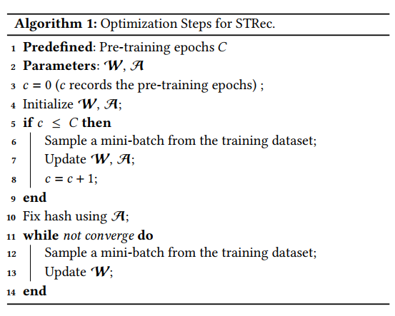
- (line 3) flag c 초기화, c를 활용해 train epoch 계산
- (line 4-9) pretrain 단계에서 모든 parameter를 동시에 train
- (line 10-14) parameter $A$를 고정하고 $W$를 train 단계에서 수렴하도록 계속 train
3.5 Model Inference
inference 과정을 순서대로 작성하였다.
- 식 $(2)$ 활용 각 interaction의 초기 representation을 만들고 $H^ 0$과 연결
- 식 $(5)$ 활용 visiting time interval $T$ 계산
- 식 $(6)$ 활용 첫 layer에 대한 index $I_ 1$ 생성
- $H^ 0$가 $L$개의 transformer layer에 의해 식 $(3)$, $(4)$와 같이 변환됨
- 식 $(7)$ 활용 각 layer $l$의 index $I_ l$이 포함된 sampling query 직접 생성
- 모든 candidate item과 sparse transformer의 output을 내적
모든 candidate item similarity 점수 $\hat{y}$을 통해 next item에 대한 prediction 결과를 획득 가능하다.
4. Experiment
Experiment setup
- Dataset
- baseline
- Evaluation Metric
Result
RQ1: How the proposed STRec performs in accuracy while it can reduce the time and spatial complexity?
RQ1에 대한 답변을 위해 accuracy 성능을 계산하여 비교한 Table 2를 제시하였다.
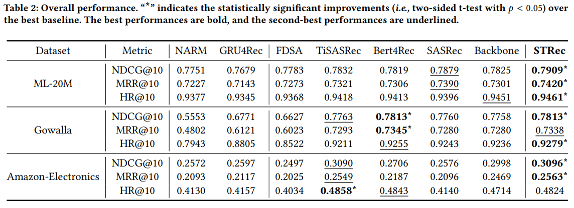
분석 결과는 다음과 같다.
- 모든 dataset에서 Transformer 기반 방법이 RNN 기반 방법보다 성능이 좋다.(긴 sequence를 더 잘 모델링하기 때문)
- FDSA는 side information이 부족하기 때문에 성능이 좋지 않다.(공정한 비교를 위해 side information 제외하고 실험)
- STRec은 65%의 sparsity를 가진 ML-20M 및 Gowalla dataset에서 다른 baseline보다 성능이 좋다.
- TiSASRec과 STRec 모두 SRS에 시간 information을 사용하였다. TiSASRec은 time interval에 따라 item embedding을 강화하기 때문에 성능이 좋지 않으나 STRec은 시간 information을 사용하여 item의 potentioal importance를 학습한다.
RQ2: Compared with the efficient transformer methods, how STRec performs in the aspect of efficiency?
RQ2에 대한 답변을 위해 efficiency performance를 측정하여 비교한 Table 3를 제시하였다.
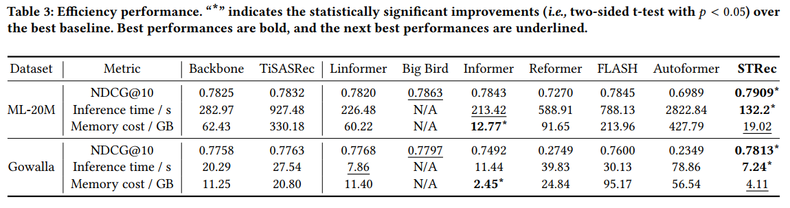
분석 결과는 다음과 같다.
- Linformer와 Informer는 backbone model보다 효율적이고, Informer는 down-sampling setting을 적용했기 때문에 가장 좋은 memory 효율을 보인다. 그러나 sampling에 많은 operation이 필요하기 때문에 STRec에 비해 inference time이 훨씬 길다. 게다가 성능도 STRec에 비해 좋지 않다.
- Big bird의 결과가 N/A인 이유는 sparse pattern에 대한 높은 complexity로 인해 효율성이 떨어져 구현할 수 없었기 때문이다.
- STRec은 시간 정보를 기반으로 중요한 query를 추출할 수 있기 때문에 accuracy와 time-space 효율성 모두에서 다른 transformer baseline들을 능가한다.
RQ3: How does the sparsity and pre-training process of STRec affect the accuracy performance?
Sparcity
Figure 4는 sparsity 측면에서의 parameter study 결과이다.
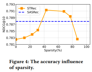
Figure 5는 sparsity 측면에서의 efficieny performance 비교 결과이다.
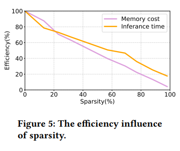
x축은 모든 layer애서의 sample size $k_ l$에 의해 계산된 sparsity를 의미한다.
e.g. sequence 길이가 50이고 $k_ l$이 5일 때 sparsity는 (50 - 5) / 50 = 90%
y축은 accuracy performance와 efficiency performance(backbone model과의 inference time과 memory cost의 percentage 비교)를 나타낸다.
Figure 4와 5에 대한 분석 결과는 다음과 같다.
- optimal sparsity는 69%이다.
- sparsity가 42%보다 낮을 때 sparsity와 model 성능은 비례한다. 그 이유는 중요하지 않은 period의 interaction에 대한 영향을 제거하여 transformer가 sequential user preference를 잘 학습할 수 있도록 중복되는 interaction 계산을 생략하기 때문이다.
- 너무 높은 sparsity는 성능을 감소시킨다. 77%보다 sparsity가 커질 때 모델 성능은 점점 감소된다. 그 이유는 sparsity가 너무 심하면 많은 key information을 잃어버리고 prediction을 충분히 학습할 수 없기 때문이다.
- (42%-77%)의 sparsity 범위에서 STRec은 SASRec(가장 성능이 좋은 baseline)의 성능을 능가한다. 그 이유는 sequence에서 representative interaction을 선택하는 성공적인 sampling 전략 덕분이다.(denoising과 비슷)
- 100%에 가까운 sparsity에서도 inference을 위한 backbone model의 cost으로 인해 I/O 및 embedding layer에도 약 15%의 시간이 소요된다. Memory cost은 주로 transformer layer에 의해 발생하므로 sparsity이 100%에 가까워지면 memory cost가 거의 0%가 될 수 있다.
Training Pipeline Analysis
Figure 6는 pretrain epoch $C$를 변화시켜 가며 실험을 진행한 결과이다.
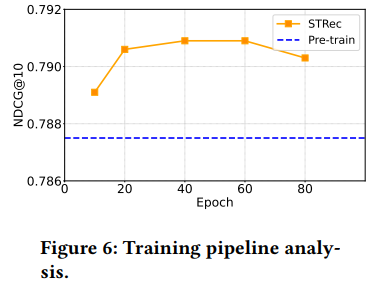
x축은 epoch $C$, y축은 performance(NDCG@10)를 의미하며
푸른 선은 fine-tuning 단계를 skip하고 바로 pre-training 단계만을 거친 모델로 예측을 진행한 결과이다.
Figure 6를 통해 다음과 같은 결과를 얻을 수 있다.
- $C$가 60일 때 성능이 가장 좋다. pre-training epoch이 그 이상으로 늘어나면 overfitting이 발생하여 성능이 감소한다.
- $C$를 60에서 10으로 감소시키면 성능은 크게 감소한다. 이를 통해 pre-training 단계를 생략하면 underfitting 문제가 발생함을 알 수 있다.
- fine-tuning 단계를 skip하면 최적의 performance를 얻을 수 없다.(blue line 참고)
RQ4: What is the influence on the performance of the core com- ponents in STRec?(Ablation Study)
Figure 7은 STRec에 대한 Ablation Study 결과이다.
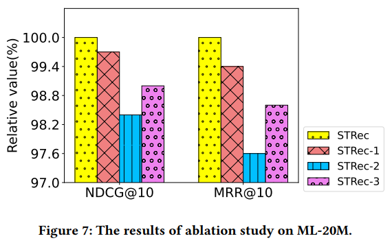
STRec에 대한 세 가지 변형으로 실험을 진행하였다.
- STRec-1 : train과 inference 둘 다에서 식 (6)의 random matrix $R$ 제거(random sampling 안함)
- STRec-2 : 식 (6)에서 index $I$를 random으로 만듦(첫번째 layer에서 item을 random으로 sampling하고 sort함)
- STRec-3 : visiting time interval matrix $T$를 item 방문 순서를 나타내는 position index matrix로 대체
분석 결과는 다음과 같다.
- STRec-1은 random sampling의 부재로 성능이 감소하였다. 모든 layer에 대한 query는 sequence의 마지막 몇개의 item으로 제한되며, 이로 인해 user interaction sequence의 초기 정보를 무시하게 되기 때문이다.
- STRec-2는 interaction을 query로 random으로 sampling하며 STRec에 비해 성능 저하를 보이는 것을 통해 sampling된 query가 interaction sequence의 random query보다 훨씬 우수하다는 것을 보여 준다.
- STRec-3의 성능 저하는 SRS에서의 방문 순서가 NLP의 단어 순서만큼이나 중요하다는 논문의 주장을 입증한다. 또한 이를 통해 SRS task에서 sampling 전략이 time interval 이외에 다른 정보를 기반으로 할 수 있음을 의미한다.
RQ5: Why the proposed method can elevate performance and shrink computation simultaneously? (Case Study)
Figure 8은 식 (9)에서의 MLP에 대한 sampling density function을 시각화한 결과이다.
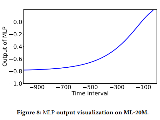
Time interval의 절대값이 작을수록 MLP의 output이 높으며 이는 sequence 뒤쪽에 가까운 interaction이 더 중요하다는 것을 의미한다.
결과적으로 현재 시점에서 가까운 interaction이 sampling될 가능성이 높으며 초기 period에서는 소수의 item만 sampling된다.
Figure 9는 user의 주요 관심사와 query로 sampling된 영화로만 구성된 첫 번째 layer의 attention weight matrix의 heatmap을 시각화하였다.
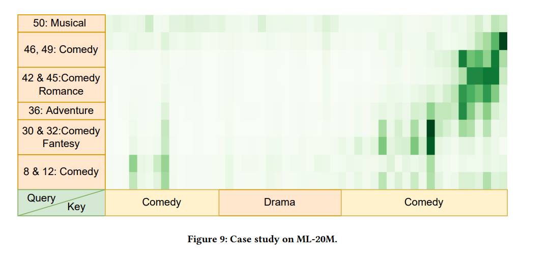
Figure 9의 Case Study는 논문의 모델이 서로 다른 period에 대해 대표 item을 추출할 수 있음을 나타낸다. 이를 통해 시간에 따라 달라지는 사용자의 다양한 관심을 나타낼 수 있다. 이러한 sampling된 item은 모델이 다양한 time period에 더 중요한 item에 집중하도록 하는 데 도움이 될 수 있다.
5. Conclusion
이 논문에서는 학습 가능한 sparse transformer인 sparce transformer for the seqeuntial recommendation(STRec)을 설계하였다.
대표 item을 선택하기 위해 모든 sequence에 대해 먼저 sampling index를
생성하는 새로운 sampling 전략을 제시하였다. 한편으로는 Cross-attention 기반 sparse transformer를 main framework로 설계하였다.
Sampling 전략을 최적화하고 정확도를 높이기 위해 STRec을 pre-train과 fine-tuning의 두 단계로 train한다.
그 결과 STRec은 inference time을 54% 단축하고 GPU memory 비용을 70%를 줄이면서도 다른 state-of-the-art 방법들보다 더 나은 accuracy 성능을 보인다.
추천시스템에서 발생하는 sparsity 특성을 활용하여 더 빠르고 memory를 적게 차지하면서도 성능이 좋은 transformer 기반 추천 모델을 제시하였다는 점이 인상깊었다.
Author Information
- SeungTai Yoo
- Contact : styoo@kaist.ac.kr
6. Reference & Additional materials
- Github Implementation
- Reference